
Analyzing SOC Data Using Jupyter Notebook
Detection Controls usually focus on telemetry collection, and in most cases lack data analytic capabilities. Hence, It would be necessary to export the data to perform data manipulation and advanced detection analytics. Jupyter Notebook is a great tool for this purpose and has no limits for what you can do with the data. Following are some of the use cases I use Jupyter in Security operations.
Working With Unstructured Data
SOC analysts tasks may involve using tools that produce unstructured to semi-structured data. To be able to analyze the data, values must be structured and parsed to appear exactly like spreadsheets. One way to do is via regex. Patterns will be identified and put in columns.
One example is Loki scanner. The tool generates one file for every endpoint. Parsing and combining all the files into one platform is the goal, especially when scanning hundreds of endpoints.Following snippet parses the rule name, the matched Yara rule and description into pandas columns from files generated with loki –csv options.
cols = ['Hostname','Type', 'File',"Rule Name","Description"]
df = pd.DataFrame(columns = cols)
row = {}

for line in lines:
    try:
        row['Hostname'] = line.split(',')[1]
    except IndexError:
        continue

    if "ALERT" in line or "WARNING" in line:
        if "ALERT" in line:
            row['Type'] = "Alert"
        elif "WARNING" in line:
            row['Type'] = "Warning"
    else:
        row['Type'] = np.NAN
    match = re.search('FILE:\s(.*?)\sSCORE',line)
    if match:
        row['File'] = re.search('FILE:\s(.*?)\sSCORE',line).group(1)

    match = re.search('Yara Rule MATCH:\s(.*?)\s',line)
    if match:
        row['Rule Name']= re.search('Yara Rule MATCH:\s(.*?)\s',line).group(1)
    match = re.search('DESCRIPTION:\s(.*?):',line)
    if match:
        row['Description']= re.search('DESCRIPTION:\s(.*?)REF:',line).group(1)

    df=df.append(row, ignore_index=True)
Once the data is represented as columns, all various analysis functions can be applied to understand the data. Complete example of using jupyter notebook with loki files can be found in this notebook.
The same can be applied to working with unparsed SIEM logs. It’s easier to export and perform analytics in Jupyter than parsing the logs in the SIEM.
Detection Rules Tuning
Detection technologies if not continuously tuned will generate high number of alerts that beat all analysts speed and energy. Another use case of Jupyter notebook is fetching and analyzing the noisy alerts data.
Working with APIs is to some extent more flexible than web portals. Qradar for example offers an API interface to work with offenses data.
offenseURL = 'https://IP/api/siem/offenses?filter=start_time%20%3E%20' + str(int(startday)) +"%20and%20start_time%20%3C%20" + str(int(endday))
crURL = 'https://IP/api/siem/offense_closing_reasons'

headers=  {
           'Range': 'items=0-100000','Version': '16.0',
           'Accept': 'application/json',
           'SEC': 'TokenHere'
          }

#offenses
ofR = requests.get(url = offenseURL,verify=False, headers=headers)
data = ofR.json()
offenses = pd.DataFrame(data)
# Closing reason
crR = requests.get(url = crURL,verify=False, headers=headers)
closeingReasons = crR.json()
Qradar represent time in Unix Epoch time. Additional column called “offense_time” will be added and contains human readable timestamps.
offenses['offense_time'] = pd.to_datetime(offenses['start_time'],unit='ms')
offenses.set_index('offense_time')
offenses['offense_time'][1]
To analyze closing reason of the fired rules, mapping the name of the reason to its ID is required since the offense API doesn’t directly replace the ID with title.
for cr in closeingReasons:
    offenses.loc[offenses['closing_reason_id'] == cr['id'], 'closing_reason'] = cr['text']
    print("ID: ", cr['id'], "   Name: ", cr['text'])
Analysis could be as simple as visualizing the escalated offenses by day or extracting most noisy offenses evidence by iterating each offense data into a dataframe.
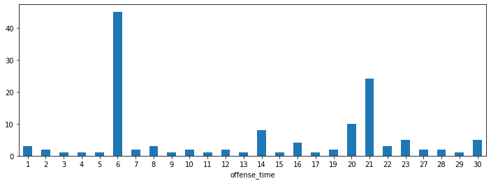
Escalated cases by day
Many other statistics can be extracted once the data is ready. As an example, number of escalated offenses each day.
fig, axs = plt.subplots(figsize=(12, 4))
offenses[offenses['closing_reason'] == 'Escalated'].groupby(offenses['offense_time'].dt.day)['id'].count().plot(kind='bar', rot=0, ax=axs)
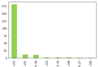
Reducing noisy evidence
Sometimes, Offenses require tuning for only one or two evidences to reduce most of the noise. Below code extracts the most noisy evidence causing offenses to fire.
# Top 10 triggered offense
Names_ofTop10 = offenses["description"].value_counts().head(10).rename_axis('description').reset_index(name='counts')["description"]
top10 = pd.merge(offenses,Names_ofTop10,on='description')

top10_by_group = top10.groupby("description")
for name, group in top10_by_group:
    fig.suptitle(name)
    #print(group["offense_source"].value_counts().head(10))
    plt.figure()
    plot_data = group["offense_source"].value_counts().head(10)
    plot_data.plot(kind="bar",color=color, label=name)
    plt.show()
    print(name)
    print("\n")
One sample output is the following graph. It’s clear that almost all offenses were fired because of one IP and if tuned, the rule FP will be acceptable.
Complete Jupyter Notebook for analyzing Qradar SIEM data can be found Here.
Time Zone Conversion
During IR engagement, data gathered may have different timezones. Using Pandas to plot or create timeline is easy with the help of to_datetime() Pandas function.Many suggest to use Coordinated Universal Time (UTC) for log analysis, but I think you should use a timestamp of most logs gathered. If most of artifacts gathered were from timezone x, then all other should be converted to the same, provided the people reading the report are located in the same timezone, otherwise UTC is preferred.
Logs with no timezone are called timezone naive, and logs with timezone are called timezone aware. First step is to ensure that all logs are timezone aware. Suggested to deal with multiple timezones by putting each timezone in its own dataframe or series.
Example:
Pandas can convert time between timezones using tz_convert() function.
time = pd . Series (['2022-04-22 08:00:00+00:00'])
utc_s = pd.to_datetime( time , utc = True )
utc_s.dt.tz_convert('Asia/Riyadh')
Similarly, tz_convert() can be used to go back to UTC.
local.dt.tz_convert('UTC')
SOC KPI and Reporting
Although, solutions such as PowerBI or SOAR are more suitable for building automated dashboard and generating reports, However Jupyter Notebooks are doing a great job with the help of visualization libraries to do the same.
KPIs are usually generated from multiple sources, especially for MSSPs where the business model deals with different solutions such as EDRs, NDRs, SIEMs …etc. Writing notebooks to automate the process worked fine. The notebook implementation will be written in a way that multiple data sources will be fetched to generate KPIs or generate reports.
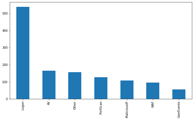
One example use case is analysis of escalated incidents by analysts. It’s sometimes not easy to directly plot the data if there is no standard for escalated tickets naming convention. Attaching tags to rows that contain specific words or match a regex can help to unify the data under standardized categories.
dfc.loc[dfc['cases'].str.contains("logon"), 'tag'] = 'Logon'
dfc.loc[dfc['cases'].str.contains("login"), 'tag'] = 'Logon'
dfc.loc[dfc['cases'].str.contains("malware"), 'tag'] = 'AV'
dfc.loc[dfc['cases'].str.contains("defender"), 'tag'] = 'AV'
dfc.loc[dfc['cases'].str.contains("symantec"), 'tag'] = 'AV'
dfc.loc[dfc['cases'].str.contains("authentication failure"), 'tag'] = 'Logon'
dfc.loc[dfc['cases'].str.contains("openssl"), 'tag'] = 'OpenSSL'
dfc.loc[dfc['cases'].str.contains("injection"), 'tag'] = 'SQLInjection'
dfc.loc[dfc['cases'].str.contains("scan"), 'tag'] = 'PortScan'
dfc.loc[dfc['cases'].str.contains("port"), 'tag'] = 'PortScan'
dfc.loc[dfc['cases'].str.contains("geo"), 'tag'] = 'Logon'
dfc.loc[dfc['cases'].str.contains("waf"), 'tag'] = 'WAF'
dfc.loc[dfc['cases'].str.contains("Intelfeed1"), 'tag'] = 'MaliciousIP'
dfc.loc[dfc['cases'].str.contains("Intelfeed2"), 'tag'] = 'MaliciousIP'
dfc.loc[dfc['cases'].str.contains("suspicious communication"), 'tag'] = 'MaliciousIP'
dfc.loc[dfc['cases'].str.contains("user added"), 'tag'] = 'UserEvents'
dfc.loc[dfc['tag'].isnull() , 'tag'] = 'Other'
Once the data is properly categorized, any aggregation method will be easily applied.
dfc['tag'].value_counts().plot(kind='bar',figsize= (11,6))
Full Notebook example for analyzing and generating KPIs of Qradar SIEM data can be found in this repository.
Advanced Detection Analytics
One interesting example is the implementation of RITA (Real Intelligence Threat Analytics) in Jupyter Notebook for beaconing detection. RITA-J is one of the examples I use to show the possibility of using Jupyter Notebook for advanced security detection use cases.